Scientific computing, from the ground up
From real‑world mathematical models to engineering solutions
The power of scientific computing and simulation.
Harish Jayaraj
Scientific Computing and Software Development Engineer
Every one of these was tested before it existed
- A bridge deck, in wind that had not blown yet
- A processor, at a temperature it had never reached
- A wing, in air it had never flown through
- A car, in a crash that never happened
Not one of them was built first and checked afterwards. They were run inside a computer until somebody was willing to sign for them.
Not one part of this was measured
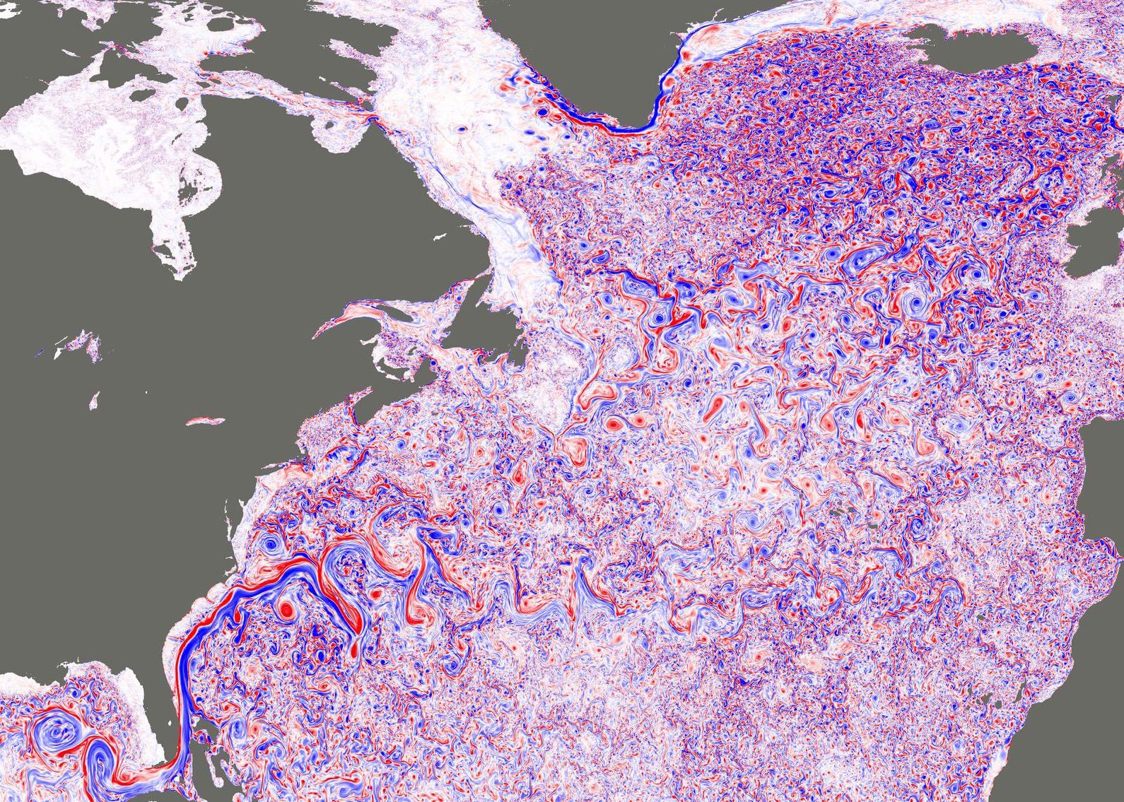
Somebody wrote down how sea water moves, and let a computer step it forward.
Not one of those eddies was drawn. They are what the arithmetic did.
The loop every one of them went through
Two of those five boxes are where the difficulty actually lives.
Box two
Model
Decide what to keep and what to throw away. Keep too little and the answer is wrong. Keep too much and nobody can solve it.
Box four
Solve
Almost nothing worth modelling has a formula. Getting a number out of an equation you cannot solve is a craft of its own.
The next ninety minutes walk that loop end to end, once, on a problem small enough to hold in your head.
Whatever you are modelling, it ends up here
A state, and a rule for how fast it changes.
Four questions, four different fields
- How hot does this chip get before it throttles?
- Will this circuit settle, or ring forever?
- How many people are infected by Friday?
- Where will the satellite be in six hours?
Different departments. Different journals. Different people, who mostly do not talk to each other.
Write each one down and they look unrelated
chip temperature
rlc circuit
epidemic
orbit
The one move that makes all four the same
A second derivative is awkward to solve numerically. So stop tracking position on its own, and track position and velocity together as a single state.
Newton's law for an orbit.
The second derivative is the problem: our methods take first ones.
Top row: the definition \(d\mathbf{r}/dt = \mathbf{v}\).
Bottom row: the original equation, because \(d\mathbf{v}/dt\) is
\(d^{2}\mathbf{r}/dt^{2}\).
Nothing was approximated, only rewritten.
Name the state \(\mathbf{u}\) and the rule
\(\mathbf{f}\).
All four models do exactly this. They land on the same line.
The shape of every model in this talk
u, the state
Every number you need to know where the system is right now. Temperature. Charge and current. Position and velocity.
f, the rule
Given the state, how fast is it changing. This is the only place your physics appears.
Which matters more than it sounds
Swap the red box and you have changed field. Everything around it is written once, tested once, and reused by everybody.
One solver simulates a ball,
an amplifier and a chemical plant.
Learn the machinery once and it pays out for the rest of your career, in whichever field you end up in.
One problem, small enough to hold in your head
You have had this since school.
Maximum range at 45 degrees.
The ball, marked at equal time intervals
Horizontal speed never changes.
Do you believe that about a real cricket ball?
What the formula quietly left out
AIR
Air resistance, in one term
The wind tunnel gives you a size. Common sense gives you a direction:
drag opposes motion. Multiply them together.
One power of the speed cancels. It is \(\lvert\mathbf{v}\rvert\mathbf{v}\), a number times a vector, not a vector squared.
Put it in the sum, divide by the mass, group the constants
Gravity's mass cancels.
A feather and a coin fall alike in vacuum.
Drag's mass does not.
It survives inside \(k = \rho C_D A / 2m\).
Now write it out in components
The horizontal equation now contains the vertical speed, and the vertical equation contains the horizontal one. They cannot be solved separately any more.
And there is no closed form.
There is no formula. So stop looking for one.
Give up knowing it
everywhere.
Settle for knowing it at \(t_0,\; t_1,\; t_2,\; \ldots\) separated by a step \(h\).
Exactness traded for existence. Every method in this act is that trade.
You already met this in your first calculus course
Taylor's theorem, exactly true.
The last term is everything you are about to throw away.
Throw it away.
You have just made your first approximation, and you know its size.
And \(\mathbf{u}'\) is exactly what \(\mathbf{f}\) hands you.
That is Euler's method.
One step, drawn honestly
The tangent is right where you are standing, and increasingly wrong everywhere else.
Drop one term of Taylor, and one step costs you \(O(h^{2})\).
Take \(T/h\) of them and the error accumulates to \(O(h)\). Halve the step, halve the error.
That is a bad exchange rate. Ten times the accuracy costs ten times the work.
Seven Euler steps at \(h = 0.6\,\mathrm{s}\), against the truth
Every step fires off along the tangent and ignores the curve bending beneath it,
so the errors all lean the same way.
The defect, once you have seen the picture
Euler trusts the slope it measured at the start of the step.
By the time the step ends, that slope is stale.
So measure it four times instead of once.
Each probe decides where the next one is taken
Two probes overshoot, two undershoot. The step takes their weighted average, and the four errors very nearly cancel.
RK4
Four evaluations of \(\mathbf{f}\) per step instead of one.
Global error \(O(h^{4})\). Halve the step and the error falls by sixteen.
Four times the work buys thousands of times the accuracy. In computing, the algorithm is worth more than the hardware.
Do not take that on trust. Measure it.
| h (s) | Euler error | ratio | RK4 error | ratio |
|---|---|---|---|---|
| 0.1600 | 2.09 m | — | 7.0×10⁻⁶ m | — |
| 0.0800 | 1.04 m | 2.01 | 4.2×10⁻⁷ m | 16.6 |
| 0.0400 | 0.52 m | 2.00 | 2.6×10⁻⁸ m | 16.3 |
| 0.0200 | 0.26 m | 2.00 | 1.6×10⁻⁹ m | 16.1 |
| 0.0100 | 0.13 m | 2.00 | 1.0×10⁻¹⁰ m | 15.9 |
2.00, row after row. 16, row after row. Not claimed, observed.
One more problem, and it is not integration
The solver marches in fixed steps. It has no idea the ground is there, so it steps straight past it.
Finding the landing is root finding: solve \(y(t^{*}) = 0\) between the two points that straddle it.
Worth the care. The integrator was accurate to \(10^{-10}\) m. Stopping at the last point throws away ten orders of magnitude in the final step.
Everything in the last act, as code
Four functions. About thirty lines.
- f the physics, and nothing else
- rk4_step one step, the four probes
- fly the loop, and where it lands
- sweep ask it the question
Nothing here is a library call you have to take on faith.
01 the physics
The first two rows are the definition of velocity. The last two are Newton's law with drag.
This is the only file you rewrite when you change problem. Everything after this slide is the same for a ball, an orbit or a circuit.
02 one step
The same four numbers back, one step later. Index 1 is y, which matters on the next slide.
The four probes from the diagram, in the order you watched them being taken.
Each line feeds the next. k2 is measured at the point k1 pointed to.
Six lines. That is the whole of the method that carries spacecraft across the solar system.
03 the loop, and where it lands
Degrees in, radians out.
The starting state: origin, speed split into vx and vy.
Work out a candidate step, but do not commit to it.
nxt[1] is \(y\). Negative means the step overshot the ground.
How far along that segment \(y\) reaches zero.
The same fraction applied to \(x\). That is the range.
The two steps that straddle the ground. nxt[1] has gone negative, so the landing is somewhere between them.
04 ask it the question
Seventy six complete flight simulations, to answer one question with one unknown.
And the answer is 42 degrees, not 45.
Hold that thought. Twenty unknowns instead of one, and this loop is why supercomputers exist.
Before you believe any of it
Turn the air off and the hard problem
collapses into one you already know.
If those two numbers disagree, something is broken, and every result after it is worthless.
This is the habit worth stealing. Find the case where you already know the answer, and check it first.
Now run it. Everything here is computed as you drag.
- Cricket ball
- Football
- Table-tennis ball
- Shuttlecock
Every point on this curve is a full flight simulation
- Cricket ball
- Football
- Table-tennis ball
- Shuttlecock
Push the speed up and watch the red peak walk away from 45.
So what is the answer?
The best angle is not 45. And it does not stay put.
cricket ball · 156 g · 72 mm · Cₔ = 0.45
| launch speed | best angle | range there | range at 45° | what 45° costs |
|---|---|---|---|---|
| 20 m/s | 43° | 33.6 m | 33.5 m | 0.04 m |
| 30 m/s | 42° | 62.9 m | 62.6 m | 0.27 m |
| 50 m/s | 39° | 118.4 m | 116.6 m | 1.78 m |
| 92 m/s | 35° | 202.5 m | 194.3 m | 8.16 m |
| 120 m/s | 32° | 241.7 m | 228.6 m | 13.09 m |
At throwing speeds, aiming at 45 costs you four centimetres.
At bowling speeds and above, it costs you metres.
Why the peak moved at all
Drag charges rent on every second you spend in the air.
A steep launch buys height, and height buys time,
and time is now something you pay for.
So the winning shot is flatter and quicker, and gets flatter the harder you throw.
Worth noticing. The peak is flat. An optimum you do not have to hit precisely is a good one, and engineers actively look for that.
Count what that answer actually cost
- 1 unknown, the launch angle
- 76 complete flight simulations
- ~4000 RK4 steps in each one
- ~1.2 million evaluations of f
All of that, and it finished before you noticed. That is the good case.
Now make it a real design problem
A wing has twenty numbers you are allowed to change, not one.
Sweeping one unknown took 76 runs.
Sweeping twenty the same way takes more runs than there are atoms in the room.
So you stop sweeping, and start using the gradient.
And our \(\mathbf{f}\) was four numbers
The loop does not change. Only the size of \(\mathbf{u}\) changes, and with it the machine you need.
This is the air a single wing throws away
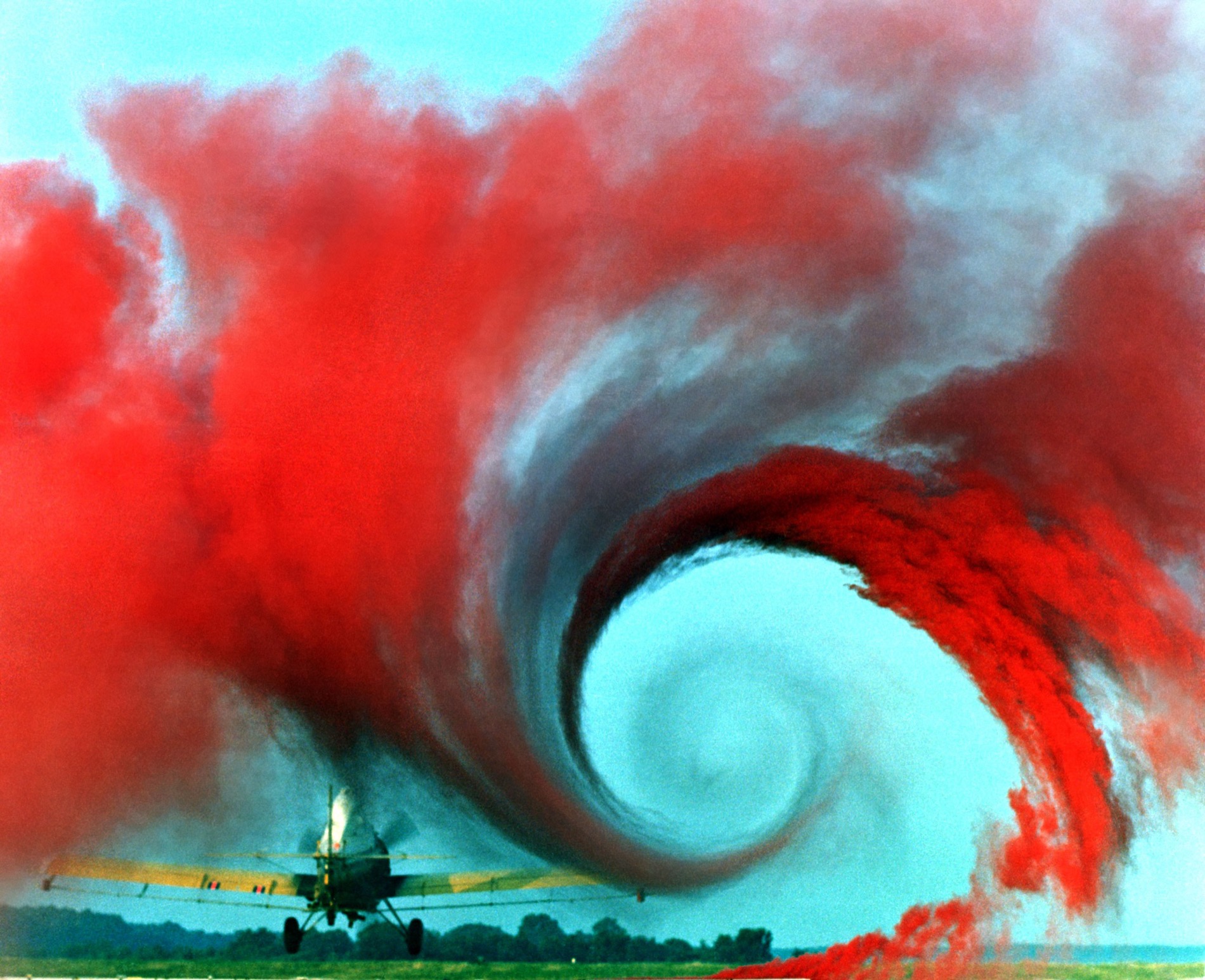
Every wing does this, all the time, and it is the reason aircraft have to be spaced out on approach.
Predicting that spiral is the same job as predicting the ball, with a great many more unknowns.
Same pipeline, different \(\mathbf{f}\)
aerodynamics
Every aircraft and every car shape is flown thousands of times inside a computer before one is built.
crash and structures
A car is crashed a few hundred times in simulation for every one crashed on a test track.
circuits
No chip is fabricated before it has been solved, node by node, step by step, in exactly this way.
weather and climate
The forecast you read this morning is the same loop, run over the atmosphere, several times a day.
None of this is new
Artillery firing tables are exactly this computation.
Angle against range, corrected for muzzle speed, air density and wind.
Produced before electronic computers existed.
One trajectory, worked by hand, took about a day.
A single table needed thousands of them.
The job title was "computer". It described a person. ENIAC, the first general purpose electronic computer, was built to do this arithmetic faster.
What the work is done with
- Python and NumPy for thinking, prototyping and plotting
- C++, Fortran, Julia when the loop has to be fast
- MPI and CUDA when one machine is no longer enough
- OpenFOAM, deal.II, PETSc when somebody has already written the hard part
You used the first one today, and hand-wrote the part the last one usually hides.
What the job actually looks like
- Decide what physics to keep, and defend the choice
- Turn it into something a machine can step forward
- Prove the answer is converged, not merely produced
- Make it fast enough to be useful to somebody waiting
- Explain the result to an engineer who will sign for it
You did the first three today, on a cricket ball.
The formula you memorised is a special case of an equation nobody can solve.
Scientific computing is how engineers work in the general case,
which is every case that has ever been built.
What you did in the last ninety minutes
- Took a question with no analytical answer
- Built a model from one law, and named what you threw away
- Built a solver, and measured its accuracy instead of trusting it
- Found an answer nobody in the room could have guessed
That is the whole working method. The cricket ball was incidental.
Take home
A different system. The same method.
A pendulum, length \(L = 1\,\mathrm{m}\), released from rest at an angle \(\theta_0\). You were given this in school:
Look at what is missing from the right hand side. The amplitude. That formula claims a big swing and a small swing take exactly the same time.
The honest model has no such claim in it:
The school formula comes from replacing \(\sin\theta\) with \(\theta\), which is only true for small angles. Put \(\sin\theta\) back and the closed form is gone.
The question. At what amplitude is the true period one per cent longer than the formula says?
Four things, one page
- One check. At \(\theta_0 = 1^{\circ}\) your period must match \(2\pi\sqrt{L/g}\) to three decimals. Run this first.
- One plot. Period against amplitude, from \(1^{\circ}\) to \(120^{\circ}\), with the school formula drawn as a flat line.
- One number. The amplitude where your curve first sits one per cent above that line.
- One paragraph. The period gets longer, not shorter. Explain why, using \(\sin\theta < \theta\).
If the check fails, stop. Nothing else means anything until it passes.
If you want more. Push the amplitude towards \(180^{\circ}\). The period grows without limit. Say what the pendulum is physically doing, and what that does to your step size.
Two things you already know how to do
The state is two numbers, angle and angular velocity. Exactly the reduction from the start of the talk.
Finding the period is event detection. Release from rest, integrate until \(\theta\) crosses zero, and interpolate the crossing. That is a quarter of a period, and it is the landing problem again.
Nothing new is required. Change four lines of what you already have and the pendulum falls out.
Send me what you build
Harish Jayaraj
Scientific Computing and Software Development Engineer
codeynamics@gmail.com
linkedin.com/in/harish-jayaraj-p
Questions.